Gradient Descent Algorithm: Key Concepts and Uses
Table of Contents

TL;DR
- Gradient descent improves model performance by adjusting parameters to reduce errors step-by-step.
- Key elements include gradients, loss functions, and learning rates for guiding models.
- Batch, stochastic (SGD), and mini-batch gradient descent each balance data usage and efficiency.
- Essential for training and fine-tuning large language models (LLMs) in NLP.
- Challenges like vanishing/exploding gradients and overfitting are managed with rate scheduling and regularization.
Diving into Key Components of Gradient Descent Algorithm

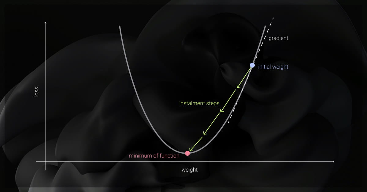
The gradient descent algorithm is foundational for expanding machine learning models. Over time, with adjustment of parameters, models reduce errors, whether we talk of deep neural networks or linear regressions. Imagine walking down a mountain in search of the lowest point; each step brings you closer to the valley. This “valley” represents the optimal error point.
Large language models (LLMs) used in natural language processing (NLP) contain millions of parameters, making gradient descent crucial for achieving high accuracy. Alongside data annotation, gradient descent ensures models learn effectively from well-labeled data.
The most common gradient descent's components include gradients, the loss function, and the learning rate.
Gradients
A gradient, simply put, is the slope or steepness of a function, and it lies at the heart of the gradient descent formula. If you were descending a mountain, the gradient would indicate the steepest direction. Gradients in a machine learning algorithm show how to adjust model parameters to reduce error or loss. By following the gradient, we can iteratively move toward the point where the model performs optimally.
Loss Functions
Feature scaling and dimensionality reduction can make gradient descent more efficient by improving convergence in high-dimensional spaces. Techniques like normalization and PCA help reduce computational cost and often enhance model performance by discarding irrelevant features.
The loss function measures the difference between a model’s predictions and actual values. In NLP models, loss functions play a significant role in training models for accuracy:
Mean Squared Error (MSE)
It measures the average squared difference between predictions and actual values, commonly used in regression problems. It penalizes large errors, making it useful for fine-tuning models with continuous outputs.
Cross-Entropy Loss
Often used in classification tasks, such as sentiment analysis, cross-entropy calculates the difference between actual and predicted probability distributions. By minimizing this loss, the model can make more accurate predictions.
Learning Rate
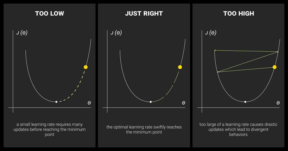
The learning rate is the step size in gradient descent and controls how big of a step the model takes in each direction. Choosing the right learning rate is crucial. Too high, and the model may overshoot the optimal point; too low, and convergence slows. Conversely, a low learning rate makes for slow progress, and while it might ensure accuracy, the model could take a very long time to converge.
Choosing the right learning rate is key, and different tasks may require different rates:
Constant Learning Rate
This parameter keeps the rate fixed across all iterations, often used in simpler models where convergence speed is not a priority. The learning rate determines how far the model’s parameters are adjusted in the direction of the gradient at each iteration.
Decay Strategies
Decay strategies use a high learning rate at the start and gradually reduce it. This helps the model make big changes at first, then fine-tune as it gets closer to the best solution. Examples include exponential decay, step decay.
Main Types of Gradient Descent Variants

There are different types of gradient descent approaches in machine learning. Different versions fit various needs, balancing stability, speed, and computational costs. Below is a breakdown of the main types and their applications:
| Type | Description | Pros | Cons | Common Use Cases |
| Batch Gradient Descent | Uses the entire dataset to compute each update | Low variance, stable convergence | Requires significant memory and computation for large datasets | Small datasets or when precision is paramount |
| Stochastic Gradient Descent (SGD) | Updates with each data point, making it faster but less stable | Faster updates, lower memory usage | High variance, may not converge smoothly | Large datasets where quick, approximate updates are useful |
| Mini-Batch Gradient Descent | Computes updates on small data subsets | Balance between speed and stability | Still requires significant memory | Widely used in LLM training where resources are a consideration |
Adaptive Gradient Descent Methods
Adaptive methods in gradient descent adjust learning rates for each parameter, which helps models find solutions more quickly and reliably. The table below compares popular adaptive methods that adjust learning rates dynamically to improve convergence:
| Optimizer | Mechanism | Strengths | Drawbacks | Ideal For |
| Momentum | Adds a fraction of past gradients to current | Speeds up convergence | Can overshoot the minimum | Deep networks |
| Nesterov Accelerated Gradient (NAG) | Anticipates next gradient for smoother updates | Accurate, reduces noise | More complex to implement | Models needing precise direction |
| RMSprop | Adjusts learning rates per parameter | Stabilizes learning | Needs decay rate tuning | Non-stationary data |
| Adam | Combines Momentum and RMSprop | Efficient, fast convergence | Sensitive to hyperparameters | NLP tasks, large datasets |
How Gradient Descent Works
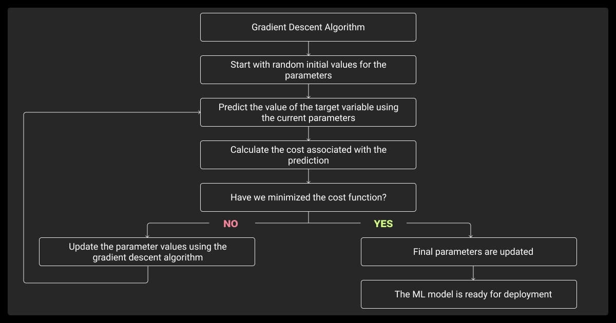
At its core, gradient descent relies on calculus and linear algebra. Gradient descent optimizes models by reducing error incrementally. Here’s a closer look at its workings:
Partial Derivatives and Backpropagation
Partial derivatives indicate how each parameter affects the loss, forming the basis of the gradient descent formula. Backpropagation then uses these derivatives to compute gradients across layers. With each backward pass, gradients are used to update weights, progressively reducing error.
To illustrate, in a neural network, backpropagation adjusts weights layer by layer, aiming to reduce the error at every iteration. This layer-wise adjustment is what enables neural networks to handle complex tasks, from understanding text in NLP to recognizing images.
Cost Function Optimization
If you look at the cost function as an area with peaks and plateaus, the goal of gradient descent is to reach the lowest peak. This is the area where a model's error is minimized. For simple linear models, this process is straightforward, but deep learning models face challenges with non-convex functions, which have multiple peaks and valleys. Advanced methods like Adam help the model navigate this complex landscape, moving it closer to the best solution while avoiding getting trapped in local minima.
Batch normalization can mitigate vanishing gradients by normalizing each layer’s inputs, ensuring stable activation distribution. This approach helps prevent the gradients from vanishing and accelerates training in high-dimensional spaces.
Uses in Model Training and Fine-Tuning

The gradient descent algorithm is vital for both training and fine-tuning complex models like transformers and LLMs used in NLP.
Training Large Language Models (LLMs)
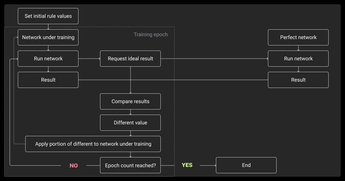
When training LLMs, batch gradient descent and mini-batch gradient descent adjust millions of parameters over multiple passes, or “epochs,” of the data. Each pass, or epoch, incrementally brings the model closer to its target accuracy. LLM fine-tuning, a step that adapts a pre-trained model for specific tasks, also relies on gradient descent.
Optimizing Parameters in NLP Models
In NLP models, gradient descent updates weights and optimizes hyperparameters, such as the learning rate and weight decay. These adjustments help improve key performance metrics, like mean average precision and recall, making the model more effective overall. This process relies on carefully prepared data annotation, which provides the labeled examples needed for accurate training and performance improvements.
The process of gradient-based hyperparameter tuning can be achieved through the following techniques:
- Grid Search: Tests all possible combinations in a predefined grid.
- Random Search: Selects combinations randomly, often faster than grid search.
Troubleshooting Common Problems in Gradient Descent
While powerful, gradient descent is not without its challenges. Let’s explore some common issues and solutions.
Managing Gradient Instability
In deep networks, gradients can either vanish (become too small) or explode (become too large), destabilizing training. In vanishing gradients, gradients diminish in earlier layers, preventing effective learning in deeper layers. Methods like gradient clipping, normalization, and smart weight initialization help tackle these problems, leading to more stable and effective training.
Learning Rate Scheduling
In training, the learning rate often needs adjustment to maintain stability. To adapt the rate, different scheduling techniques can be used:
- Step Decay: Lowers the learning rate at intervals to enhance stability in later stages.
- Cosine Annealing: Gradually reduces the learning rate in a smooth curve for refined adjustments.
In high dimensions, gradients can shrink to near-zero, slowing convergence, or explode, causing instability. Using adaptive optimizers like Adam can help maintain stability by dynamically adjusting learning rates.
Overfitting and Regularization
Overfitting happens when a model starts picking up on random noise in the data instead of the true underlying patterns. This reduces its accuracy on new data. To combat this and adapt to the real-world use, several techniques are used, such as L2 regularization, dropout, and data augmentation
Practical Examples of Gradient Descent in Action

Here’s how gradient descent techniques are applied in real-world scenarios:
Example 1: Training a Transformer Model with Adam Optimizer
In training a transformer for text classification, the Adam optimizer’s adaptive learning rate speeds up convergence. With an initial learning rate of 0.001, Adam achieves better accuracy than SGD, making it popular in NLP tasks where time and precision are crucial.
Example 2: Optimizer Comparison on a Classification Task
Each optimizer has strengths and trade-offs that affect training speed, accuracy, and stability. In a sentiment analysis task, comparing these optimizers reveals which one best suits specific needs.
| Optimizer | Convergence Speed | Final Accuracy | Stability | Best Use Case |
| SGD | Moderate | 82% | Moderate | General-purpose, large datasets |
| Adam | Fast | 88% | High | NLP, quick tuning |
| RMSprop | Moderate | 85% | High | Non-stationary data |
Example 3: Fine-Tuning a Language Model with Mini-Batch Gradient Descent
Mini-batch gradient descent in LLM fine-tuning processes data in chunks, balancing memory use and computational efficiency. This approach is ideal for LLM fine-tuning in task-specific NLP applications, like named entity recognition, enabling fast adaptation to particular needs without overloading resources.
Gradient descent is crucial in machine learning, as it refines models to enhance accuracy and efficiency. More than just a method, it’s the backbone of transforming data into reliable insights and predictions. For anyone working with NLP and AI, mastering gradient descent is key to effective training and model success.
About Label Your Data
If you choose to delegate data annotation, run a free data pilot with Label Your Data. Our outsourcing strategy has helped many companies scale their ML projects. Here’s why:
Check our performance based on a free trial
Pay per labeled object or per annotation hour
Working with every annotation tool, even your custom tools
Work with a data-certified vendor: PCI DSS Level 1, ISO:2700, GDPR, CCPA
FAQ
What happens if the learning rate in the gradient descent algorithm is set too high?
A high learning rate can cause the model to overshoot the optimal point, leading to erratic parameter updates. This often disrupts convergence and creates instability in training.
What is the basic formula for gradient descent?
The basic formula for gradient descent is: θ = θ - α∇J(θ). Here θ represents the parameters, α is the learning rate, and ∇J(θ) is the gradient of the cost function. This formula helps to minimize error.
What is the best gradient descent algorithm?
The best gradient descent algorithm depends on the task, but Adam is widely favored for its adaptive learning rates and quick convergence, especially in deep learning and NLP tasks. Its versatility makes it a top choice for many applications.
What are the three main types of gradient descent algorithm?
The three main types of a gradient descent algorithm are batch gradient descent, stochastic gradient descent (SGD), and mini-batch gradient descent. Each type differs in how much data it uses per iteration, balancing precision, speed, and computational efficiency.
Written by
Karyna is the CEO of Label Your Data, a company specializing in data labeling solutions for machine learning projects. With a strong background in machine learning, she frequently collaborates with editors to share her expertise through articles, whitepapers, and presentations.


