3D Computer Vision: How It Works and Where It’s Used

Your perception stack runs LiDAR at 10 Hz, your daytime model performs well in urban driving, and you still miss partially occluded pedestrians at 60 meters. Sound familiar? 

3D computer vision sits at the core of every modern autonomy stack, and almost every team building one runs into the same walls. This article walks through how 3D CV actually works and where it gets deployed. It also covers why data pipelines are usually where things break.

What Is 3D Computer Vision?

3D computer vision is the set of techniques that give machines a sense of depth and spatial geometry. It uses structured representations of the physical world, built from sensor inputs like LiDAR, stereo cameras, and radar.

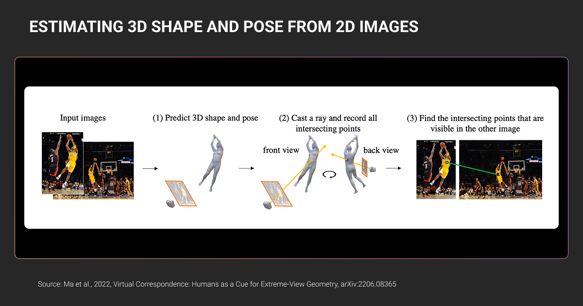
The distinction from 2D CV matters for your architecture. A 2D model predicts bounding boxes on a pixel grid. A 3D model predicts object position, size, orientation, and velocity in metric space, usually in a bird’s-eye-view (BEV) frame or world coordinates.

That shift from pixels to meters changes what downstream components can do. Path planning needs metric truth. So does collision avoidance. Trajectory forecasting breaks down without accurate depth, and multi-sensor fusion requires every detection to live in a shared spatial frame.

How is 3D computer vision different from 2D?

Two things change in practice: the data and the evaluation.

In 2D CV, your pipeline consumes RGB frames at 30 or 60 FPS. Models like YOLO, DETR, or Mask2Former predict 2D boxes or masks. Ground truth comes from human annotators labeling images. A mid-size dataset is millions of images, and a skilled annotator can label a frame in seconds.

In 3D CV, your pipeline consumes point clouds, often at 10 Hz, plus time-synchronized camera and IMU data. Models like PointPillars, CenterPoint, TransFusion, and BEVFormer predict 3D cuboids with nine parameters: x, y, z, length, width, height, yaw, and two velocity components. Ground truth comes from annotators working in 3D space across synchronized modalities. A single labeled LiDAR sweep for a dense urban scene takes significantly longer than any 2D frame, typically an order of magnitude more.

That gap is the first thing most AI and ML teams underestimate.

How Does 3D Computer Vision Work?

3D computer vision works in three layers:

1. The sensor layer captures geometry
2. The representation layer structures the data
3. The perception layer interprets it

Every production autonomy stack builds on this foundation, with variations by sensor suite and deployment domain.

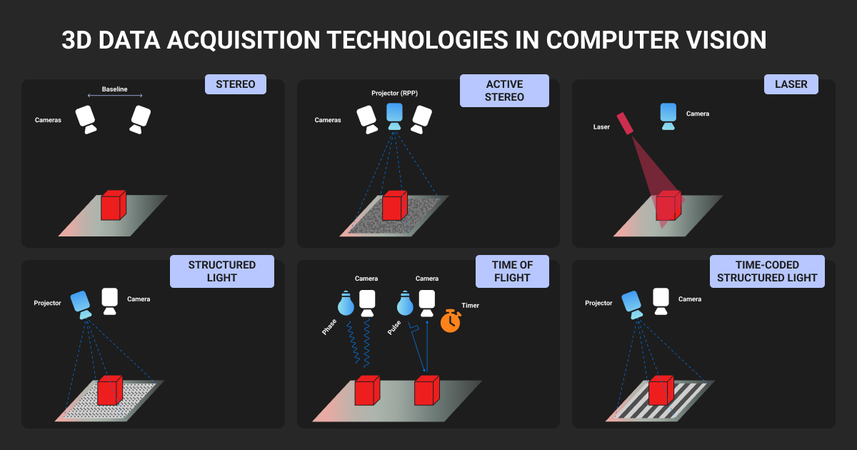
What sensors feed 3D computer vision?

Four sensor types show up most often in vision 3D perception stacks.

LiDAR

Time-of-flight laser sensors that produce point clouds with direct depth measurements. Typical automotive LiDAR outputs 64 to 128 beams at 10 Hz, producing 100,000 to 500,000 points per sweep. Accuracy is centimeter-level in good conditions. Range varies widely by unit, from around 100 meters on older rotating scanners to 200+ meters on newer solid-state designs from vendors like Luminar, Innoviz, and Ouster.

Stereo cameras

Two cameras with a known baseline compute depth by triangulation. Depth accuracy degrades quadratically with distance, which is why stereo works well up to about 30 meters and falls off past that. NODAR’s Hammerhead system and Mobileye’s SuperVision rely heavily on stereo. It’s cheap, camera-native, and struggles in featureless scenes.

Time-of-flight (ToF) cameras

RGB-D sensors like Intel RealSense or Microsoft Azure Kinect. Dense depth at short range (1 to 5 meters). Dominant in indoor robotics and warehouse automation, with overlap into logistics.

Radar

Measures range and velocity directly via Doppler shift. Long range and weather-robust, with sparse output. Radar has had a 4D renaissance since 2023 with high-resolution imaging radar from Arbe, Mobileye’s imaging radar roadmap, and Continental’s ARS540, producing dense enough point clouds to support direct 3D detection.

Each sensor covers for the weaknesses of the others. That’s what sensor fusion is for.

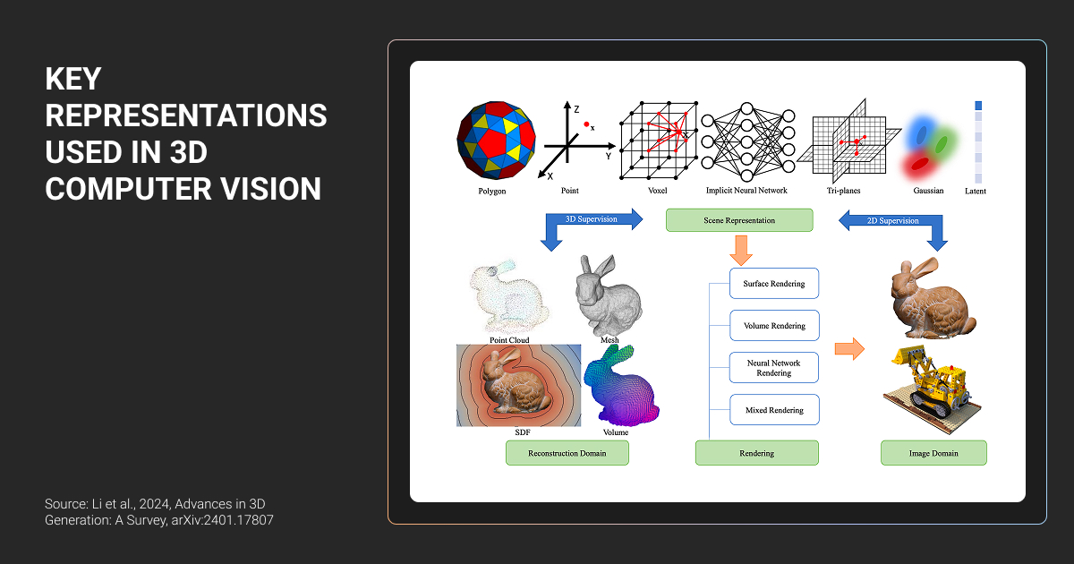
How is 3D data represented?

The representation you choose affects your computer vision 3D model choice and your training budget. It also shapes your data annotation workflow. 

Four formats dominate:

• Point clouds. Unordered sets of (x, y, z, intensity) points. Native LiDAR output. Used by PointNet, PointNet++, and PointPillars.
• Voxel grids. Point clouds discretized into 3D cells. Used by VoxelNet, SECOND, and CenterPoint.
• Bird’s-eye-view (BEV) feature maps. A top-down 2D projection with per-cell features encoding height and density. Used by LSS, BEVFormer, BEVFusion, and most modern multi-modal stacks.
• Range images. LiDAR data projected onto a 2D cylindrical grid. Fast to process, with some geometric loss. Used by RangeNet++ and several Waymo internal models.

BEV has become the dominant representation for production AV stacks, largely because it lets you fuse camera and LiDAR features in a shared top-down space that maps cleanly to planning and control.

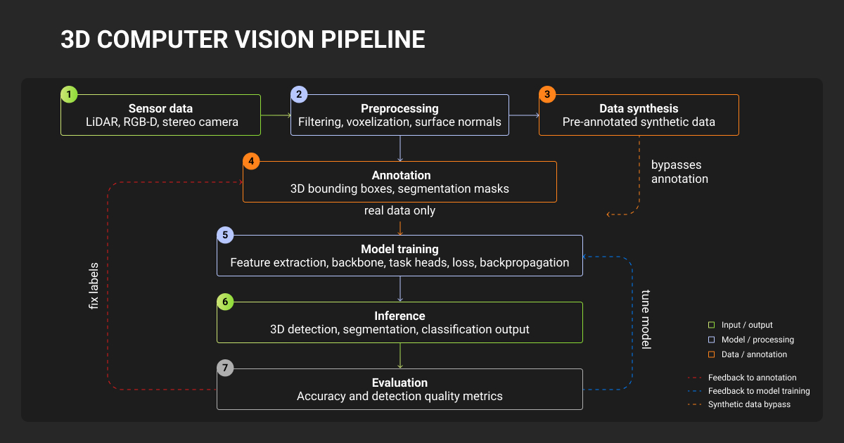
What does the 3D perception pipeline look like?

A typical 3D perception pipeline runs six stages:

1. Synchronization. Time-align LiDAR sweeps, camera frames, radar packets, and IMU data to millisecond-level accuracy.
2. Calibration. Apply intrinsic and extrinsic matrices to put every sensor in a shared coordinate frame.
3. Preprocessing. Remove ground points, downsample the cloud, accumulate multiple sweeps for temporal context.
4. Detection. Predict 3D boxes for vehicles, pedestrians, cyclists, and other classes.
5. Tracking. Associate detections across frames to produce stable object IDs and velocity estimates.
6. Fusion. Combine detections from LiDAR, camera, and radar into a unified object list.

Most engineering teams spend their cycles here. Each stage has its own failure modes, and each stage depends on labeled data that matches the stage’s assumptions.

Pro tip: If your tracker drops IDs between occlusions, the problem is rarely the tracker. Check whether your training set includes enough occluded object annotations with consistent track IDs across frames. Most open datasets don't.

Where Is 3D Computer Vision Used?

3D machine vision powers perception in every domain where a system has to navigate, manipulate, or inspect the physical world. The dominant deployment contexts today:

Autonomous vehicles and ADAS

This is the flagship use case and the largest buyer of 3D perception data. Full-stack AV developers like Waymo, Zoox, Pony.ai, and Wayve run multi-sensor perception stacks with LiDAR, cameras, and radar. ADAS programs (Mercedes Drive Pilot, GM Super Cruise, Tesla Autopilot) increasingly use 3D perception even in camera-only stacks, often through learned depth estimation and BEV feature lifting.

Typical data needs: 3D cuboids for vehicles, pedestrians, and cyclists, multi-frame tracks, panoptic segmentation, lane annotations, traffic light state, and scenario tags.

Autonomous trucking

Kodiak Robotics, Waabi, Aurora, Gatik, and Plus operate highway perception stacks where detection range is the primary constraint. At 70 mph, a truck covers 31 meters per second, so a 300-meter detection horizon gives you roughly 10 seconds of reaction time. Long-range 3D object detection is existential for this segment.

Outdoor delivery robots

Starship, Serve Robotics, Kiwibot, Coco, and Nuro deploy in unstructured pedestrian environments. Sensor suites are smaller (often stereo plus a low-cost LiDAR or solid-state unit), and detection ranges are shorter. The edge-case distribution is also long-tailed. Curb detection and sidewalk segmentation dominate the label taxonomy, with vulnerable road user classification close behind.

Warehouse and industrial robotics

Autonomous forklifts (Third Wave Automation, Vecna) and pick-and-place robots (Covariant, RightHand Robotics) use RGB-D and stereo for bin detection and free-space mapping. AMRs like Locus and 6 River Systems apply the same stack to object pose estimation. Object pose annotation here is 6-DoF, and the data is heavy on CAD-aligned labels.

Drones and aerial systems

Drone inspection for infrastructure (Skydio, Percepto, DJI Enterprise) relies on photogrammetry and dense 3D reconstruction. Agriculture and mapping drones produce orthomosaics that get annotated for crop health, boundary detection, or asset inventory. Labeling here sits between traditional 3D annotation and geospatial workflows.

Vehicle inspection and damage detection

Tractable, Ravin.ai, and UVeye use multi-view imaging and structured light to produce 3D models of vehicles for damage detection. Insurers and rental fleets are the primary buyers. Annotation blends 3D surface segmentation with part classification.

What Are the Main Challenges in 3D Computer Vision?

3D vision in computer vision is hard because physical-world data is messy, sensors disagree, and every edge case has to be encoded into the training set. 

Four challenges consistently stall perception teams:

Sensor fusion

Fusion fails when sensors disagree. Disagreement usually comes from one of three sources: 

• Miscalibration (extrinsics drift with temperature and vibration)
• Desynchronization (a 20ms timing offset moves a 70 km/h vehicle 39 cm)
• Representational mismatch (your camera detects a pedestrian while the LiDAR beam passed above their head)

Modern architectures like BEVFusion and TransFusion handle some of this in the model itself, learning cross-modal attention that can compensate for small calibration errors. Your training data still has to include the disagreements you want the model to resolve. If every frame in your training set has perfectly aligned sensors, the model won’t know what to do when calibration drifts in production.

This is where data annotation pricing starts to bite. Annotators have to work across synchronized camera and LiDAR views, and when the views disagree, the human has to decide what’s actually there.

LiDAR data quality

LiDAR point clouds are sparse by design. Point density falls off quickly with distance. A pedestrian at close range returns a manageable cluster of LiDAR points; the same pedestrian at 100 meters returns only a handful. Your model has to decide whether a tiny scatter of points is a pedestrian, a traffic cone, or noise.

Weather adds further failure modes. Rain creates spurious returns from water droplets. Fog scatters the beam. Snow occludes ground points. Most open datasets like nuScenes, Waymo, and KITTI are dominated by clear-weather daytime data, and models trained on them degrade sharply in adverse conditions.

Teams that deploy in cities with real weather end up running targeted data collection campaigns and investing heavily in weather-specific annotation.

Long-range detection

Long-range 3D detection is a known-hard problem for a simple reason: the number of points returned from an object drops with roughly the square of distance. A vehicle up close returns hundreds of points. At 120 meters the same vehicle returns far fewer. At 200 meters, the target can be reduced to a sparse handful.

Annotation at long range is equally hard. Annotators working from LiDAR alone struggle to disambiguate a vehicle from a large sign at 150 meters. Camera-assisted labeling helps, but the camera itself resolves fewer pixels on a distant object.

The practical effect: your long-range detection performance is usually limited by your long-range label quality. Swapping the model architecture rarely changes that.

Occlusion and partial visibility

Real scenes are full of partial objects. A pedestrian behind a parked car. A cyclist emerging from behind a truck. A vehicle visible only through its wheels under a barrier. Production models have to handle these cases, which requires training data that includes them, labeled correctly and consistently.

The hardest annotation calls sit at the occlusion boundary: how much of an object has to be visible before it gets labeled? How do you annotate a vehicle whose bumper is visible while its body is hidden? Different guidelines produce different models. Teams that change guidelines midway through a project end up with inconsistent training sets and perception regressions.

The biggest challenge in building 3D computer vision models is handling occlusions and depth perception in dynamic outdoor scenes. Cluttered construction sites bury objects behind equipment or vehicles, confusing 2D-to-3D mapping and spiking errors up to 40%. One geo-fenced event site case dropped alert inaccuracies by 70%, enabling instant remote interventions.

Chris Edens Owner, Mobile Vision Technologies

Why annotation becomes the bottleneck

Add these four challenges together and the annotation cost compounds.

A 2D bounding box takes an annotator seconds. A 3D cuboid on the same object takes minutes. The annotator has to fit the box in three dimensions across synchronized sensor views and check it from multiple viewpoints. When LiDAR and camera evidence disagree, they also have to resolve the disagreement. A full scene with dozens of objects tracked across a multi-second sequence can absorb hours of annotator time per sequence, plus annotation QA.

This is where most in-house teams stall. You hire an annotation lead and build out a team of 5 to 10 annotators. You invest in data annotation tools, and six months later, your data throughput is still the limiting factor on model iteration velocity.

Tooling is rarely the bottleneck. What matters is the combination of trained annotators, consistent guidelines, multi-sensor QA, and the throughput to keep up with fleet data collection. Point cloud annotation is one of the genuinely hard ML ops problems, and it usually doesn’t get solved in-house. We’ve seen this pattern enough times that we stopped being surprised by it.

This is the part of the pipeline where specialist data annotation services earn their fee. Two Label Your Data case studies are representative.

Ouster, the digital LiDAR sensor maker, needed precise 3D cuboid and 2D bounding box labels across static and dynamic sensor deployments, feeding a performance regression pipeline that informed their sensor software releases. 

We started in December 2020 with a two-person team and a dedicated project supervisor who wrote the annotation guide before anyone else touched the data. The team scaled to ten annotators over the project’s lifespan, and a 10% turnover rate kept the label-guideline knowledge intact as the work grew. Ouster’s product performance went up 20% on their own benchmarks. MOTA improved 15%. F1 reached 0.95. None of that came from a model architecture change.

The precise LiDAR annotations and consistent quality from Label Your Data, even as the project scaled, have been invaluable, significantly boosting our product performance and ML accuracy.

Dave Pike Senior Engineering Manager, Ouster

NODAR, which builds stereo-based 3D depth perception for autonomous driving, industrial automation, and agriculture, needed dense polygon masks for supervised depth training. Public datasets didn’t cover their sensor-specific edge cases. 

Our team delivered roughly 60,000 labeled polygon objects across roads, terrain, vehicles, people, and airport equipment, at 1-2k images per dataset with a 3-to-4-week turnaround. The workflow stayed the same from pilot task to parallel production. Every batch opened with documented guidelines and a live training call, and a QA feedback loop caught drift before it contaminated downstream batches.

The pattern in both cases is the same: separate the annotation pipeline from the core ML team. Your engineers work on models. A dedicated team at a data annotation company works on labels, with QA tuned to the 3D modality. Written guidelines travel with the team when it scales, and a feedback loop catches drift early.

Practical Tips for 3D Computer Vision Data

Five things to think about before your next annotation cycle:

1. Capture data in the conditions your model will actually see. Most open machine learning datasets are clear-weather daytime. If you deploy in Seattle or Detroit, your training set needs rain, snow, and low-sun-angle frames.
2. Budget 3D annotation as a major cost line. Equivalent 3D work commonly runs many multiples of 2D cost. Planning at 2D rates is the most common failure mode in early-stage perception programs.
3. Invest in sensor calibration before you scale data collection. A 0.5-degree extrinsic error on a camera produces a 1-meter ground-truth error at 100 meters. That error propagates into every label.
4. Label dynamic objects as tracklets. A consistent object ID across frames is more valuable than a slightly tighter box on any single frame.
5. Standardize your occlusion guidelines early and freeze them. Every mid-project guideline change creates label drift your model will learn.

Pro tip: If you’re about to scale a perception dataset past six figures of labeled frames, audit your label consistency first. Pull a few hundred frames at random and re-annotate them with a different team using the same guidelines. Then measure agreement. Most teams discover their first-pass agreement is worse than they assumed and realize they need to rewrite the guidelines. Better to find that early than late.

Where 3D Computer Vision Goes From Here

3D vision technology has moved from research to production in under a decade. The sensor economics keep improving, with automotive-grade LiDAR moving from a premium niche component toward a viable commodity for volume platforms. The model architectures keep getting better at fusing modalities. BEV is converging as the production representation.

What hasn’t changed is that the data pipeline is where most projects succeed or fail. The teams shipping reliable 3D perception are the teams that treated labeled data as a first-class engineering problem, with the same rigor they apply to model training and infrastructure.

About Label Your Data

If you’re scaling a 3D annotation pipeline or evaluating a specialist partner for LiDAR, sensor-fused, or long-tail perception labeling, the Label Your Data has delivered programs like Ouster’s and NODAR’s for clients in AV, trucking, industrial robotics, and maritime. We’re always open to a technical conversation about data strategy, even if you’re not ready to outsource yet.

No Commitment

Check our performance based on a free trial

Flexible Pricing

Pay per labeled object or per annotation hour

Tool-Agnostic

Working with every annotation tool, even your custom tools

Data Compliance

Work with a data-certified vendor: PCI DSS Level 1, ISO:2700, GDPR, CCPA

FAQ

What is a point cloud in 3D computer vision?

A point cloud is an unordered set of 3D points, each defined by x, y, z coordinates plus optional attributes like intensity or RGB color. LiDAR sensors output point clouds natively, producing hundreds of thousands of points per sweep. Unlike images, point clouds have no fixed grid structure, which is why models like PointNet and PointPillars use architectures built for variable-size, permutation-invariant input.

Can you do 3D computer vision without LiDAR?

Yes. Camera-only stacks use monocular depth estimation, stereo triangulation, or multi-view geometry to infer depth from RGB frames. Tesla, Mobileye, and NODAR all operate without LiDAR. The tradeoff is range: camera-derived depth degrades quadratically with distance, so long-range detection suffers. Most camera-only deployments compensate with larger datasets and temporal models that accumulate depth across frames.

How much labeled data do you need to train a 3D perception model?

It depends on the architecture and domain. Public benchmarks give a floor: nuScenes has about 40,000 keyframes, while Waymo Open Dataset has roughly 200,000. Production AV teams train on millions of labeled frames. Narrower domains like warehouse robots can work with tens of thousands, especially when fine-tuning on pretrained models. Label quality and edge-case coverage usually matter more than raw volume.